2D graph
The Dewesoft 2D graph shows the drawing of any vector channels. Some typical examples are FFT created from math channels, classification and others.

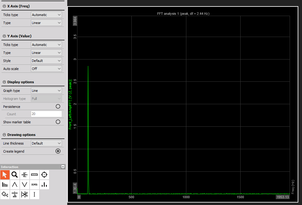
When you select 2D graph, the following settings will appear on left and right part of the screen:
- Control properties - For detailed information about Control properties: grouping, number of column, Add / Remove, transparency —> Instrument appearance.
- Drawing options - Selects which parameters will be shown on the graph
- Channel selector
The input to the 2D graph can be:
- FFT math
- STFT math
- CPB math
- classification
- counting
- scope trigger
- FRF math
- SRS math
- CA pressure and other channels
In short, 2D graph can show any array channel created by Dewesoft.
Properties
There are several properties which can be set to 2D graph.
Auto-scale - will automatically scale y axis
Graph type - Automatic will set the graph type to what is set in the input channel. For example, FFT has the default graph type of lines while CPB has histogram. We can override these settings by manually defining either Lines or Histogram.
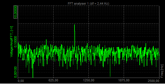
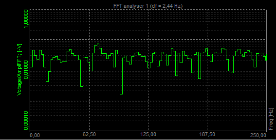
- Histogram type - for histogram type, we can define to either fill the bars with Full option, or to draw empty bars with Empty option or to simply draw the Line at the top for a very classical instrument look. Full histogram:
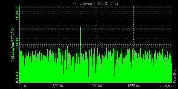
Empty histogram:
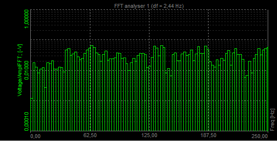
Line histogram:
- X Axis type - can be either linear or logarithmic
- Y Axis type - can be either linear, logarithmic, Amp dB where the 0 dB is the full scale or Power dB
- Number of ticks - defines either automatic or manual number of graph divisions for x and y axis. Division for y axis can be freely defined only for linear scaling, log scaling defines number of ticks from minimum and maximum axis value.
- Single value axis - will set one y axis scale for all channels in the graph
- Persistence - will slowly fade the old data on the graph. We can define number of old arrays to be shown. The larger the number, more history will be seen. Persistence graph:
Interaction
The 2D graph can display values of the currently selected point with the markers. When clicking on such point with the right mouse button an option to add marker is shown.
Manual about processing markers can be found here.
The type of markers:
- free marker
- max marker
- harmonic marker
- sideband marker
- RMS marker
- damping marker
- kinematic marker
- vector cut marker
Free marker
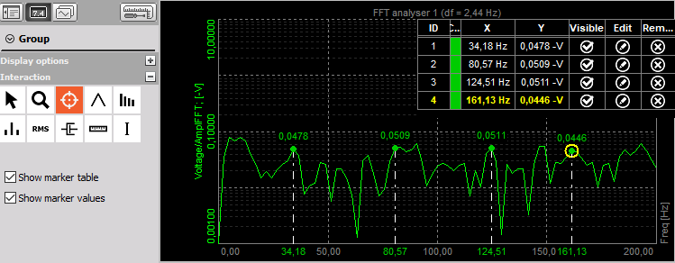
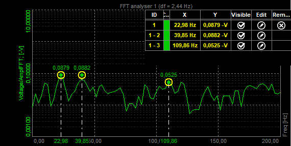
Free markers can be freely added. Marker shows us frequency of the peak at which it stands and its amplitude. With Show marker table selected you can see the table of markers - its ID, type, channel, color, its frequency (X-axis) and its amplitude (Y-axis). You can select if you want markers to be visible or not, you can also edit and remove it.
Max marker
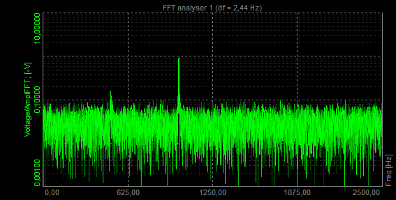
Max marker finds the highest amplitude in the spectrum.
When we select Max marker and click on the FFT graph with the left mouse button the following setup opens.
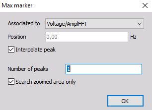
First, we select the FFT curve to which the marker is related to. The position is calculated by the program. Depending on the selected window type, the frequency component (actual peak) can fall in between two adjacent lines. Then we select a number of peaks we want to find. If that number is 1 program will only find the peak with maximum amplitude. If that number is 2 it will find also the peak with second highest amplitude. The picture below shows the max marker with 2 number of peaks selected.
Harmonic marker
The harmonic marker is a great help when identifying the fundamentals of the frequency.
The harmonic marker can be enabled at any frequency. The harmonic marker will mark the harmonics of the selected frequency. The base marker of the harmonic marker can be selected and moved to any other frequency with the harmonics updated live.
Then select the base frequency with the mouse and add a harmonic marker with the click on the left button.
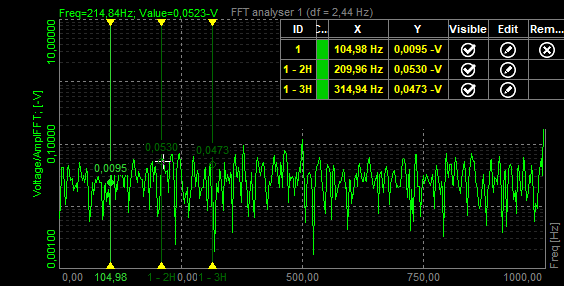
We select the first peak at 104.98 Hz. If we select Number of harmonics as 3, we will see lines at 104.98 Hz, 209.96 Hz (2 x 104.98 Hz) and at 314.94 Hz (3 x 104.98 Hz). And the theoretical harmonics also nicely match with our measurement results - first three harmonics are nicely seen.
You can also pick and drag the fundamental frequency through the FFT spectrum. Harmonics will automatically follow.
Sideband marker
Sideband marker monitors the modulated frequencies to the left and right from the selected center line.
Let’s generate an amplitude modulated signal with a carrier frequency of 1000 Hz and the base-band signal with a frequency of 100 Hz.
Sideband markers have a center marker and several equally spaced sideband markers. By selecting the center marker, you can drag the sideband markers to different positions while still maintaining the individual sideband space.
Each sideband cursor can be selected and moved to a different frequency hence changing the individual ratio of the side bands with respect to that of the center cursor.
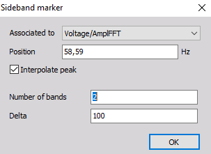
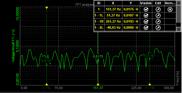
Sideband marker draws markers around the selected peak. We have to define the Number of bands (for how many bands in each direction we want to see drawn lines) and Delta (distance between bands in Hz). For example, selected position is 1000 Hz, a number of bands is 1 and Delta frequency is 100.
We can see that the central position is at 1000 Hz and we have one band in each direction. So the line on the left side is at 900 Hz and line on the right side is at 1100 Hz. Distance between the lines can be defined by the user, in our example it was 100 Hz.
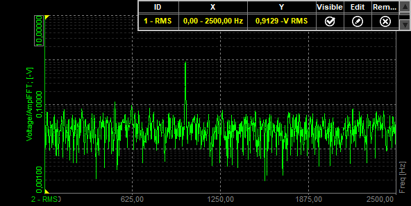
RMS marker
RMS marker will sum up all the FFT lines in the selected band and calculates the RMS value.
RMS marker calculates RMS value of the channel between cursors or between defined area.
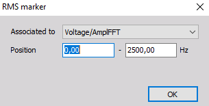
The RMS value of the channel between cursors can also be adjusted by dragging cursor with a mouse. RMS will be calculated automatically if the area changes.
Damping marker
Damping markers are best to use in modal testing when we want to find out how our transfer curve is damped. We select it when we are interested in the quality factor, damping ration or attenuation rate of a selected peak.
Then click on the mouse button to the position, where you want to add a damping marker.
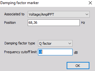
When selecting the damping marker the following setup appears:
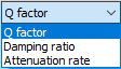
Damping factor type can be selected from the following options:
- Q factor
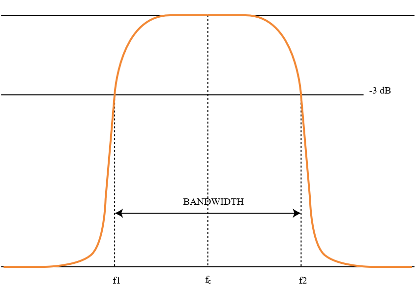
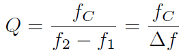
The Q (quality) factor of the damped system is defined as:
The higher the Q, the narrower and ‘sharper’ the peak is.
- Damping ratio - Damping ratio and quality factor Q are related through equation:

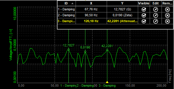
- Attenuation rate - Attenuation is the gradual loss in intensity of any kind of flux through a medium. It is usually measured in units of decibels per unit length of the medium. In the picture below we can see a transfer curve of a beam. On each of the peak, we attach a damping factor and in the marker table we can see the quality factor (Q), which tells us, how much the transfer curve is damped. If Damping factor type is chosen as Damping ratio, the result is Zeta for each peak. If Damping factor type is chosen as Attenuation, the esult is attenuation ratio for each peak.
For more information about processing markers please take a look at the manual that is avaialble here.