FIR Filter setup

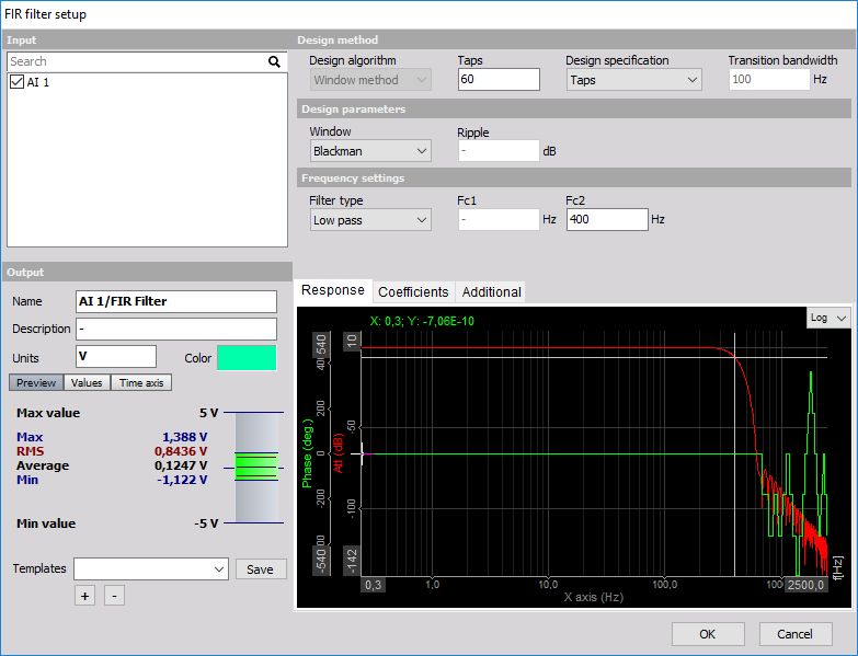
When you press the Setup button on newly activated FIR Filter line, the following FIR filter setup window will open:

The filter supports multiple input channels.

For detailed information about basic settings of the input and output channels see  -> Setup screen and basic operation Math.

FIR stands for finite impulse response. In theory, it means that the response to the impulse will be zero after some time (exactly after the samples will equal to filter order).

Another nice property of the filters is that basically phase response is linear. The phase shift in time is half of the number of samples if the filter is calculated for the samples in the past.

Since Dewesoft has calculation delay, we can use a trick to compensate the filter delay and have absolutely no phase shift in pass as well as in the transition band of the filter. This is a major benefit compared to the IIR filter where we always have a phase shift. The drawback of FIR filters is that they will use more CPU power compared to IIR.

We will make a comparison between these two types a bit later; now let’s take a look at basic properties how to set the filter.

FIR Filter settings

For FIR Filter you can set:

• Design method
• Design algorithm
• Window method (for now)
• Design specification
• Taps / Order
• Transition bandwidth
• Design parameters
• Window type
• Blackman
• Rectangle
• Hamming
• Hanning
• Kaiser - Ripple
• Flat top
• Frequency settings
• Filter type
• Low pass
• High pass
• Band pass
• Band stop
• All-pass (Hilbert)
• Additional
• Scale

You can see the effect of this setting directly on Response curve / Coefficients preview  for Filter type: Low pass, High pass, Band pass, Band stop and different Window type:

Filter type

You can select Filter type from list between:

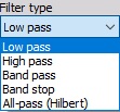
• Low pass - Low pass filters cut the high frequencies of the signals.
• High pass -High pass filters DC and low frequencies.
• Band pass - Band pass filter filters high and low frequencies, so there is only one band of values left.
• Band stop - Band stop filter filters only one section of frequencies.
• All-pass (Hilbert) - An all-pass filter is a signal processing filter that passes all frequencies equally in gain, but changes the phase relationship among various frequencies

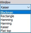
Window type

You can select Window type from the list. The window defines the behavior of the filter in the transition and the stop band (the height of the sidebands and the width of the main band). For common usage, Blackman window is quite good choice, because the side bands are extremely low.

Taps / Order

In this field, you can enter Taps.  The taps of the filter define the number of coefficients of the filter and that will directly affect the slope of the transition band. The filter taps are not directly comparable with FIR filter. 

Transition bandwidith

In this field, you can enter the Transition bandwidth. The Transition bandwidth defines a range of frequencies that allows a transition between a passband and a stopband of the filter. The transition band is defined by a passband and a stopband cutoff frequency. In the following example a 100 Hz Cut of frequency was chosen with 100 Hz Transition bandwidth.

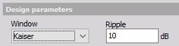
Kaiser window type - Ripple

When a Kaiser Window type is selected, new Ripple field appears on the right side of the Window type field. In this filed you can enter ripple value in dB. It tells the maximum allowed pass band ripple of the filter. The more this value is, the bigger will be non-linearity in the pass band, but the filter will be steeper.

Cut-off frequency

The filter cutoff frequency defines the -6 dB point (half amplitude) of the filter. You can enter the Cut-off frequency in the field:

• Fc1  - Low  frequency (You can enter Fc1 for Low pass, Band pass and Band stop filter).

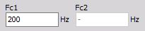
• Fc2 - High frequency (You can enter Fc2 for High pass, Band pass and Band stop filter).

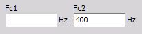
• Both High and Low  frequency (You can enter Fc1 and Fc2 for Band pass and Band stop filter).

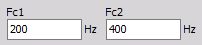
Fc1 value must be always lower than Fc2. These values are limited by filter stability. In Dewesoft the filters are calculated in sections, which enable the ratio between cutoff and sample frequency in a range of 1 to 100000. So we are able to calculate 1 Hz high pass filter with 100 kHz sampling rate.

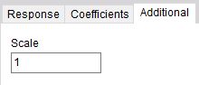
Scale

For filters, you can enter also Scale. Scale factor means the final multiplication factor before the value is written to the output channel. It helps us to change the unit, for example. A good example of using the Scale is shown in the Integration section.

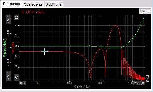
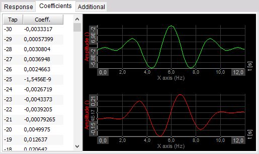
Response curve / Coefficients preview

You can choose between Response curve preview and Coefficients display.

The red response curve shows the amplitude damping of the filter. The amplification ratio is expressed in dB (similar to IIR filter). The green curve shows the phase delay. In the pass band as well as in the transition band the phase delay is always zero and in the stop band the phase angle is not even important because of high damping ratio.

The other display is the display of coefficients. The upper graph and the left table shows the filter coefficients with which the raw data is convoluted. The lower graph shows the response of the filter to the step response.

On Response curve preview you can choose between Logarithmic and Linear display, you can also edit coordinates value and auto scale Yaxis.

Filter comparison

Let’s look at the difference of the FIR filter compared to the standard IIR filter. Let’s take a very simple 20 Hz second order filter (at 1 kHz sampling rate).

The IIR filter is calculated with 6 coefficients, while similar FIR filter is calculated with 40 coefficients for the same damping. Therefore the FIR filter is more CPU demanding for the same performance.

Another fact is while we can get ratios of cutoff frequency to sample rate of 1/100000 and more, we can achieve only limited results with FIR filter. The ratio increases with the higher number of coefficients.

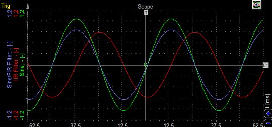
Enough of the downsides, let’s look at the response graph at 20 Hz (exactly at the limit). The green curve is the original sine wave while the red one is calculated with IIR filter. We can clearly see the phase delay of the output.

The blue curve is the response of the FIR filter which has absolutely no phase shift. For lots of applications, it is very important that the signals are not delayed and there the use of FIR filters is very advantageous.