Modal geometry
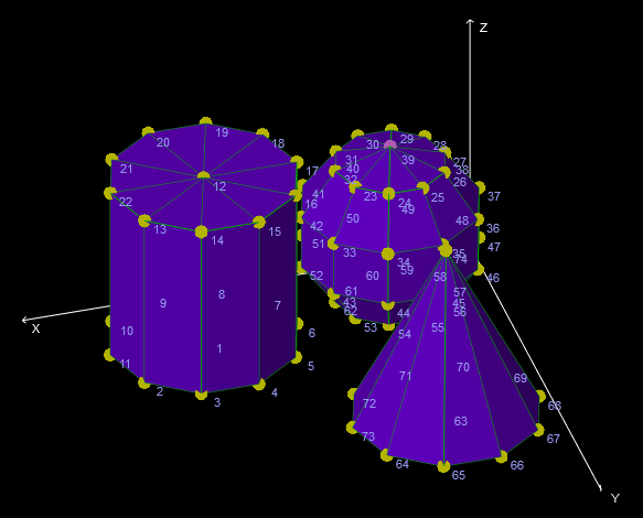
Structural geometries can be imported or created in the Modal Geometry display widget. This module is also integrated into the Modal Test and Time ODS setup modules, where the Geometry editor has its own tab section.
For more information about Modal test take a look at the Modal test and analysis manual.
The Modal geometry visual control widget is used to visualize animation of the structure. It can be found under the Machinery diagnostics section of the Widgets list.
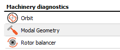
If the icon does not appear, the visual control Modal Geometry.vc must be added to the Addons folder under the Dewesoft program files folder.
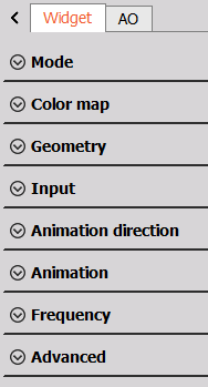
The Modal geometry widget has a longer list of widget properties as shown below. These will be described in the following sections.
Geometry settings
Model source
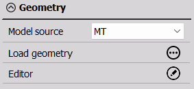
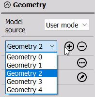
Under the Geometry section the Model source determines which of the available geometries that will be used.
If you have multiple applications that include the use of a geometry, then you can select between which one of them to animate.
For example, if you work with the Time ODS module and you have created a geometry in the Time ODS module setup, then you can select to use it here under Modal source.
If you haven’t created a geometry already in some module then you can select the User model and then Load or create a new geometry for that specific widget.
Load and edit geometries
Geometry can be loaded from UNV file format or Edited manually.
- Load UNV - Loads structure data from external UNV (universal file format) file
- Edit - Opens Modal Geometry/UNV editor. The Editor is described under the section UNV Editor.
Mouse controls on the geometry:
- Left click: rotate structure
- Right click: translate structure
- Left+Right click: zoom
- Mouse wheel: zoom
Widget view mode settings
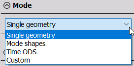
The modal geometry widget view settings found in the header of the widget. The view settings are dependent on the selected view Mode setting. The available view Modes will depend on which modules that are included in the current used setup. Some of them are:
- Single geometry
- Mode shapes
- Time ODS
- Custom
Visibility
In common for all view Modes are the widget Visibility settings:
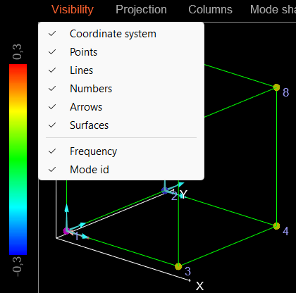
Icons in the Visibility section are used to enable/disable the items listed below:
- Coordinate system - The global coordinate system
- Points - Node points
- Lines - Tracelines, that connects nodes
- Numbers - Node IDs
- Arrows - Orientation arrows for the current measured group of DOFs
- Surfaces - Defined surfaces
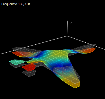
- Frequency - The frequency related to current animation
- Mode ID - The mode shape number (only shown for the Mode shapes view Mode)
Projection
Depending on the view Mode, different projections are possible. For example, when selecting Single geometry view Mode, then both 3D, 2D, and multiple XYZ projections are available as shown below:
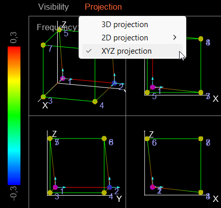
Whereas for the Mode shapes view mode the multiple XYZ projections are exchanged with multiple mode shapes animated at the same time.
By using the Custom Mode you can have multiple different geometries in a single widget, where you can select the Model Source for each added geometry:
In most cases the Single geometry view Mode or Mode shapes view Mode is the right one to use.
Color map
The color map property defines the colors used across the animated deflection interval. A wider range of color maps can be chosen between, and some of them are illustrated in the picture below:
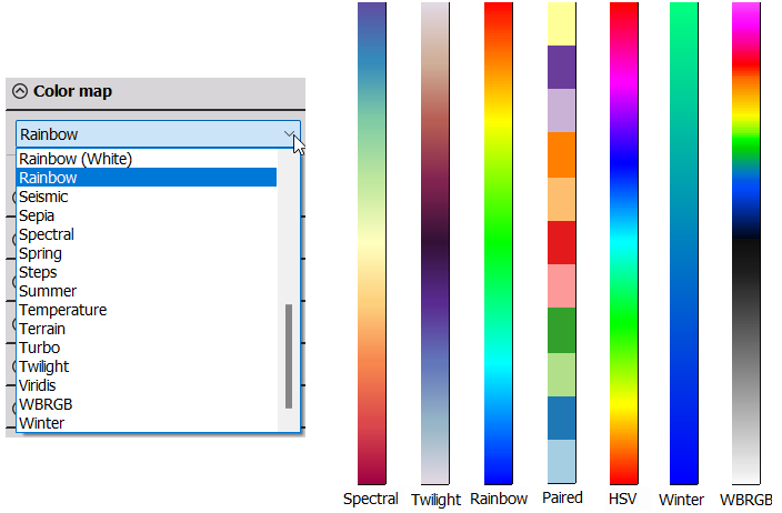
Rainbow is selected as the default Color map.
Input
The Input settings determine which data results that should be used for the animation.
First, the Transfer function setting is used to select which function type to use. This could e.g. be FRF H1, FRF H2, ODS FRF, or Mode shape.
If you only have results for one of the supported function types then that will be shown automatically:
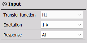
The Excitation and Response drop-down properties determine the group of DOFs to animate and which phase reference that will be used.
For example, in the picture above the Input settings are set to animate All responses relatively to the phase of the Excitation at Node ID 1 in the X direction.
Note: For mode shapes the Input settings are disabled since mode shapes can use all Excitation- and Response measurement for estimation of modal models including the mode shapes. The modal analysis estimation process can use the phase information from multiple reference DOFs to determine one model, and hereby both All Excitations and All Responses are used.
Animation direction
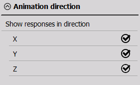
The Animation direction gives you the ability to visualize the animation in a reduced number of directions.
If All Responses have been selected under the Input section, then it will be the response DOFs that you reduce the animation directions for. In the same way, if All Excitations have been selected under the Input section, then it will be the excitation DOFs that you reduce the animation directions for.
Animation
At the Animation section you have different ways to manage how the geometry will be animated:
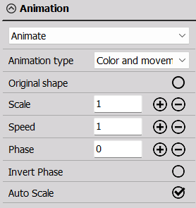
First you can select between if you want the geometry to move or stand-still at a fixed position. You can select between:
- Animate - structure will be moving/animating
- Max Shape - the geometry is fixed at the max deflection phase position
- Manual - the geometry is fixed at a user-defined phase position.
Animation type
The animation can be selected in different representations:
- Movement
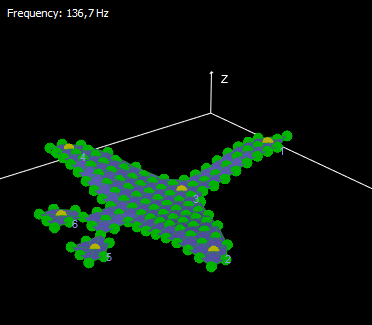
- Color
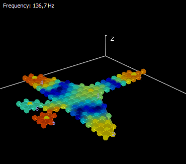
- Color and movement
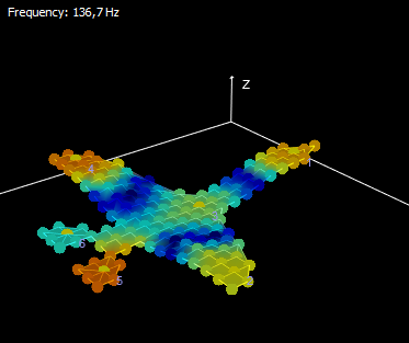
Show original shape
By checking the Show original shape checkbox, the undeformed structure will be shown (grayed out) at the same time as deformed one.
Scale, Speed, and Phase
Scale and Speed values define how fast and how much nodes should move. Default value for both fields is 1.
The Phase can be used to look at the structure at a certain deflection position, but it can also be used to align the phase of two different modal geometry animations. For Max Shape animation the Phase parameter is not shown.
Auto-scale
With Auto-scale enabled, the animation will automatically scale the color map and deflections such that the geometry moves with similar amplitudes when changing what should be animated - for example, when changing the frequency for a MT animation. This is often used for FRF and mode shape animations where you animate relative magnitude deflection levels.
If the Auto-scale is disabled the color map and deflection range will stay fixed, such that the geometry will vary how much it moved when changing what to animate. This is often used for ODS FRF animations where you animate absolute amplitude deflection levels.
Animation at selected frequency
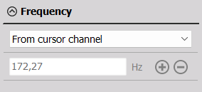
Animation of the structure is done at a defined frequency. This frequency can be defined:
- From cursor channel - animated frequency is taken from yellow cursor on 2D graph
- Manual - manually define animated frequency
Advanced
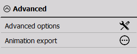
Under the Advanced settings section you can:
- Modify the animation processing even further under Advanced options,
- Export a video of the animation under Animation export
Advanced options
In Modal geometry, also the unmeasured points can be animated. They must be connected with a line to a measured point in order to animate them.
We do the animation of the unmeasured points with interpolation, and the interpolation settings are user-defined.
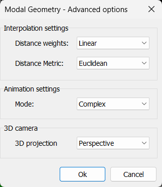
In most cases the Distance weights should be set to Quadratic and the Distance Metric to Euclidean, in order to animate the structure in a way that relates the most to real life dynamic movements.
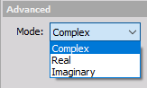
Animation settings FRF’s calculated from the Modal test module are complex channels. They contain information about amplitude, phase, real and imaginary parts. To support this, we can also animate the real, imaginary or complex part.
Animation export
The animation can be exported to a video file, which makes it easy to share and use in various presentations.
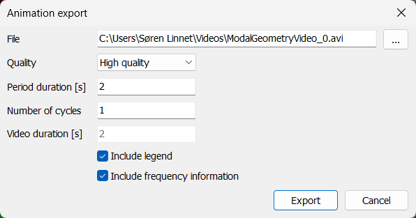
The Period duration will determine the speed of the moving geometry in the animation.
The Video duration indicates the full time length of the video based on Period duration and Number of cycles.
UNV Editor
Explanation of terms
For easier understanding, main terms are explained here.
- Object - pre-defined object in geometry (cuboid, circle, plate, …)
- Node - Node is point on the geometry, where a sensor might or might not be mounted. Nodes are defined with a Node ID, location (X, Y, Z) and rotation around axes (X angle, Y angle, Z angle).
- Line - Line connects two nodes together.
- Surface - Surface can be defined with 3 or 4 nodes
- Cartesian coordinate system - Usually nodes are presented with a Cartesian coordinate system. This means you have X, Y, Z position and rotation around all three axes. Coordinate system can be used for grouping nodes, because you can later rotate or translate them with a Center point.
- Cylindrical coordinate system - Cylindrical coordinate system is used for easier creation of round objects. Points are defined with radius, angle and z (height) around coordinate systems center point.
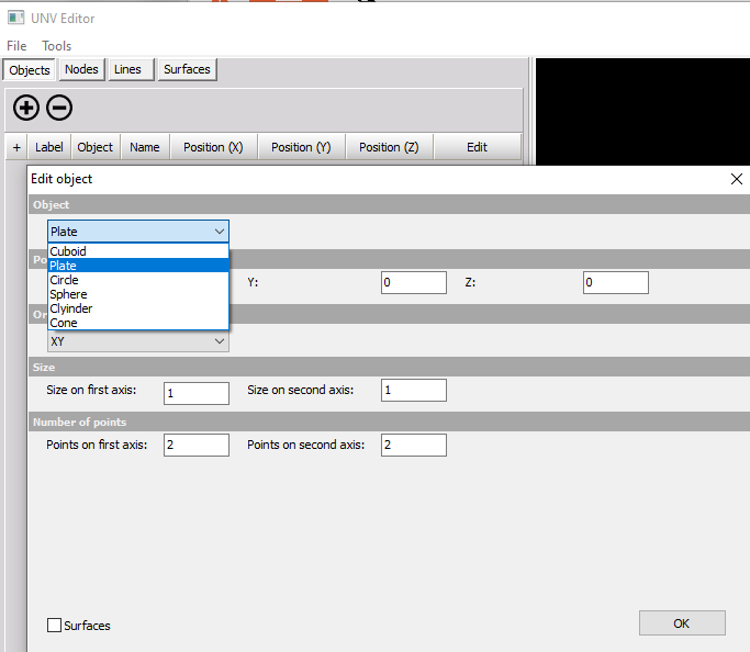
Objects
The structure can be assembled from pre-defined objects. The object that are available in Geometry are:
- Cuboid
- Plate
- Circle
- Sphere
- Cylinder
- Cone
For each object you can define the position (X, Y and Z coordinate), size (of axis) and number of points in each axis.
If the user selects the option Surfaces, then surfaces will automatically be assigned to the structure.
Nodes
In order to create a new structure from nodes, we have to switch to the Nodes tab. Now we have to create a coordinate system in which we will define our nodes. This can either be Cartesian or Cylindrical.
After the coordinate system is created, we can add nodes with the Plus button.
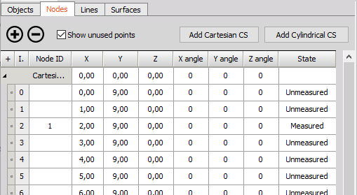
When a node is selected, we can also remove it by pressing the Minus button on Nodes tab.
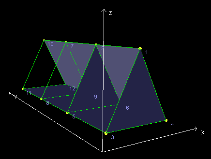
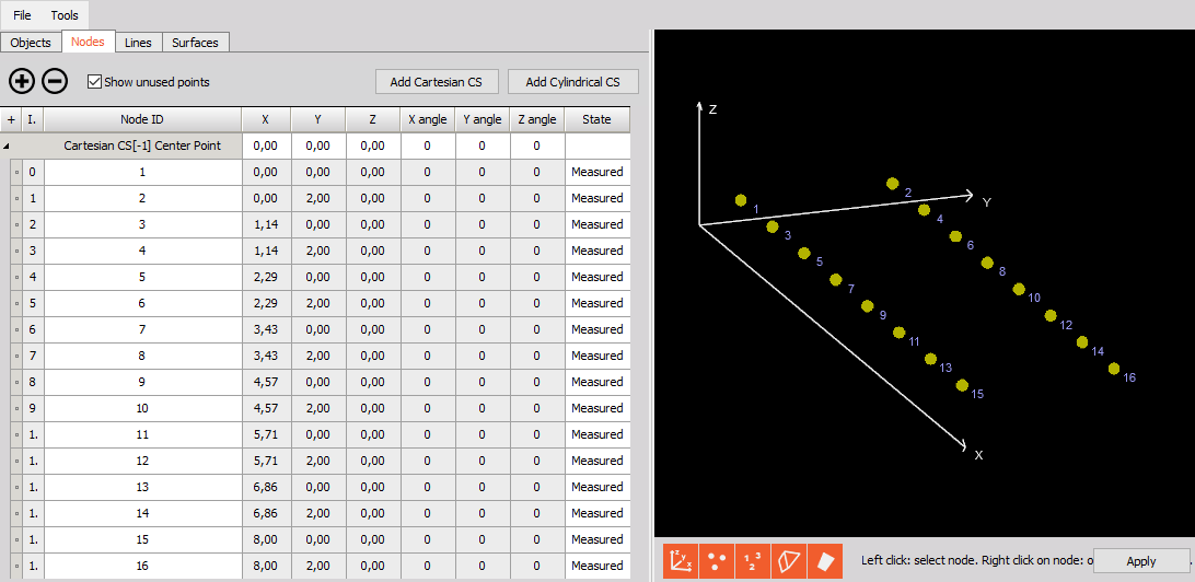
In the picture below, you can see the Cartesian coordinate system with 16 nodes.
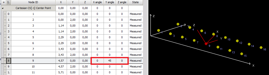
After nodes are created we can change their rotation (according to how the sensor is rotated on the object) with all three axes. Nodes can be selected with selection in the Nodes table or by right-clicking on the structure preview window. When a node is selected its local node rotation is shown with a local coordinate system located directly on the node. In the picture below you can see a selected and rotated node.
Rotation convention
Node rotations can be defined with many different conventions. In the Modal geometry editor the rotation convensions supported are the so called Intrinsic x-y’-z” or Extrinsic z-y-x Tait-Bryan angles which represents rotations about three distict axes.
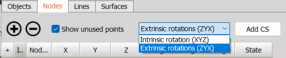
Intrinsic - means that the rotations occur about the axes of the rotating node or coordinate system xy’z”.
Entrinsic - means that the rotations occur about the axes xyz of the original coordinate system, which is assumed to remain motionless.
If you already have rotated nodes defined by 3x3 matrices, maybe generated by a Coordinate Measuring Machine (CMM), and want to determine the angles to type in, in order to rotate nodes such that they have similar rotations, then you can use the intrinsic and extrinsic formulas below:
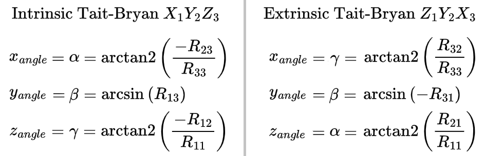
where R_xx is the normalized coordinate element of the rotated node matrix.
As an example, below you see three nodes with lines representing a rotated coordinate system for a node. In order to rotate a new node into having similar rotations as visualized by the node lines, you can use the formulas above and type in the resulting angles for the new node:
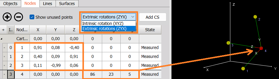
In the picture above the new node with Node ID 4 has its local CS directly on the node lines to the other nodes.
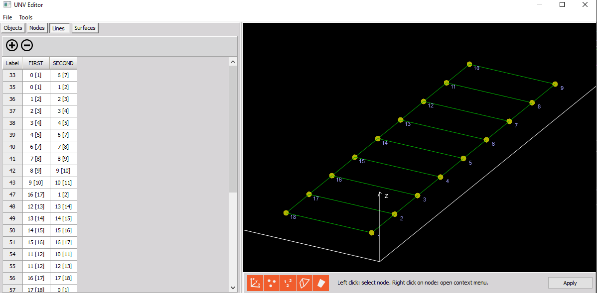
Lines
When nodes are defined we can go ahead and add lines to connect them.
Easiest way to create lines is to right click with the mouse on the node, select Add -> Lines.
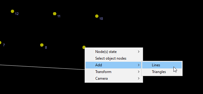
Left click on the first node and move to the second node. This will create a white line and when you hover to the node, the line will change to green color. Select the second node and the line will be added.
You can add mulsitple lines consecutively.
Right mouse click will stop adding lines
If we don’t want to draw connecting lines by clicking on the animated nodes, we can also manually add lines by pressing on the Plus button under the Lines tab.
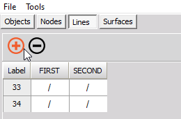
When a new line is addedto the Lines table we have to select the nodes which the line will connect – we can do that with selecting nodes in the table.
In the picture below we can see an object with some trace lines added.
Surfaces
Triangle surfaces can be added with a right mouse click, Add -> Triangles.
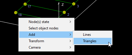
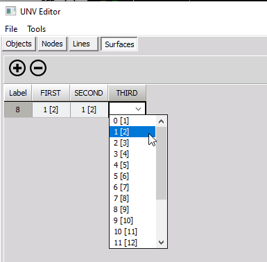
In order to add a triangle surface, 3 points must be selected as shown in the image below.
Triangle surfaces can also be added by clicking the plus button and manually defining corners.
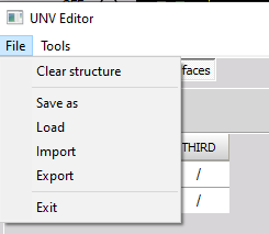
Additional options
- Clear structure - the whole structure will be cleared
- Save as - save the geometry as an XML file
- Load - load existing XML file into the editor
- Import - import UNV/UFF files
- Export - the structure can be exported to UNV/UFF file format
- Exit - option will close the UNV editor and discard all your changes
.
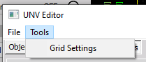
Grid
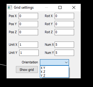
Under Tools -> Grid settings a grid can be added into the coordinate system.
You can define the position, rotation, orientation and size of the grid.
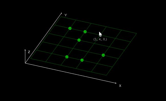
The grid is displayed in the coordinate system.
By pressing the CTRL button on the keyboard and left click on the mouse, you can add a node to a grid.
By default, the node is set to unmeasured (green color).
Node(s) state
Nodes state can be:
- Measured - point in the structure that we measured. The color of the point is yellow.
- Unmeasured - point in the structure that was not measured. In order to animate unmeasured points, it must be connected with a line to a measured point.
- Hidden - hidden point in the structure
Transform
- Move
- Rotate
- Scale
Object
- Group - group selected nodes into an object
- Ungroup - ungroup selected object into nodes
- Duplicate - duplicate selected nodes/objects
- Delete - delete selected nodes/objects
Camera
- Set anchor point to selected node - the anchor point of projection, will be placed to the selected point