Decimator
The Decimator math module can be used to downsample/reduce the sample rate of selected synchronous channels.
Downsampling can be useful for certain synchronous channels e.g. if such channels are only relevant to measure with a fraction of the sample rate of the Analog Input channels.
With a reduced sample rate the data usage of stored files will also be reduced, but the decimated data will also only contain reduced signal information with a frequency span up to a fraction of the used input signal frequency span.
The Decimator math module supports both IIR and FIR based decimation and simple linear sample reduction.
Add the Decimator module to a setup
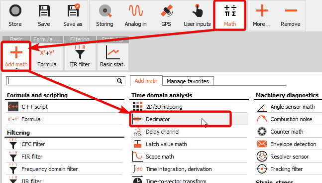
The decimator module can be added to a setup by clicking the Add math button under the Math tab, and then select the Decimator module which can be found under the Time domain analysis section:
Decimator module setup
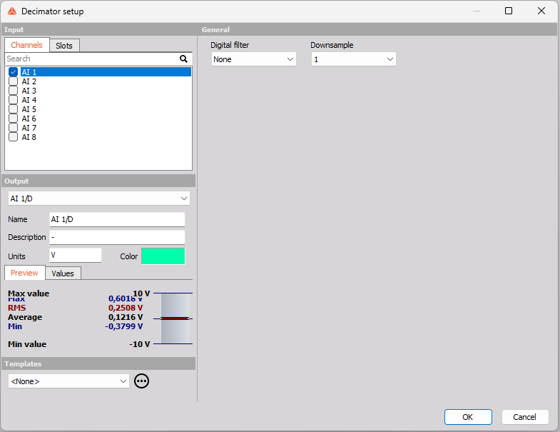
After adding a Decimator math module, or when clicking on Setup for such a module, then you will get a setup screen for the module, like illustrated below:
Downsample
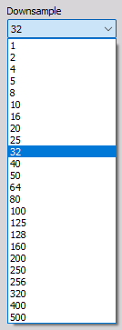
The Downsample parameter determines the decimation factor.
For example, having an Input channel with a sample rate of 100 kHz and the Downsample parameter is set to 20, then the decimated output sample rate will be 100 kHz / 20 = 5 kHz.
The Downsample decimation factor can be set to one of the values in the dropdown list illustrated below:
Digital filter
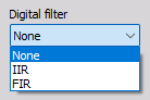
The decimation process can be performed either by using a decimation IIR or FIR filter or instead by using the option ‘None’ which performs linear sample reduction:
A Digital IIR or FIR decimation filter can be applied to eliminate aliasing effects. Aliasing effects will appear if the input channel contains signal components at frequencies above the Nyquist frequency of the decimated output channel. The Nyquist frequency is half the related sample rate.
Applying an IIR or FIR Digital decimation filter will also add Low-Pass filtering which will remove signal components above the decimated Nyquist frequency before the decimation process is performed. Hereby all signal components that would have caused aliasing are removed.
With Digital filter set to None no low-pass filtering is applied.
An example for why to use a decimation IIR or FIR filter
As an example let’s say the input channel has a Sample rate of 5 kHz and hereby a Nyquist frequency of half of that being 2.5 kHz. The signal content in that channel includes a sine tone at 2.4 kHz. Now we decimate that channel with a factor of 2, which makes the processed output channel have a Nyquist frequency of 1.25 kHz. The new Nyquist frequency is below the frequency of the sine tone at 2.4 kHz and therefore that tone can not be described correctly.
Based on the fundamental theory of signal processing, the new decimated signal will still try to include all the signal information that was in the original signal, but all components above the new Nyquist can not really be that and will instead be reflected back and forth across the frequency axis.
The 2.4 kHz tone end with showing up at 100 Hz when illustrated in a FFT spectrum as shown below:
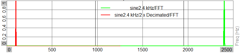
With a new Nyquist of 1.25 kHz the 2.4 kHz tone reflects back a frequency amount of 2.4 kHz - 1.25 kHz = 1.15 kHz, and going 1.15 kHz back from Nyquist make the component end up at: 1.25 kHz - 1.15 kHz = 0.1 kHz, as we see by the red graph.
IIR settings
If the Digital filter is set to IIR, then related IIR settings will appear in a section as illustrated below:
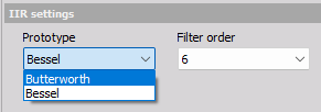
Prototype
Butterworth can be selected for better linear amplitude behavior whereas Bessel can be selected for a better linear phase behavior.
Filter order
The Filter order determines the steepness of the low-pass filtering. The amplitude level will attenuate with about -20 dB per Filter order over a frequency decade. For example a 4th order IIR filter will attenuate with -80 dB per decade.
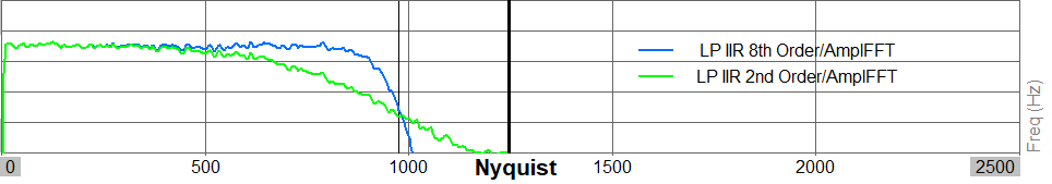
As illustrated above, the greater the filter order is the greater the frequency range will be where you still have a linear amplitude response before the filter begins attenuating.
IIR filter cut-off frequency
The cut-off frequency used for the digital IIR low-pass filtering is set equal to the decimated sample rate divided by 2.5. For example if a channel with a 5 kHz sample rate is decimated with a factor of 2, then the LP-filtering will have a cut-off frequency at 2.5 kHz / 2.5 = 1.0 kHz.
At the cut-off frequency the LP-filtering will provide an attenuation of -3 dB.
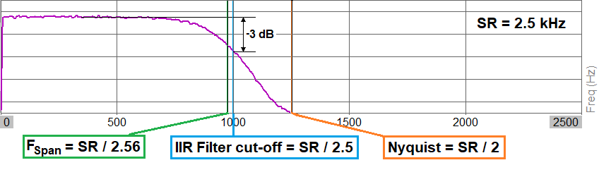
Note: The frequency at the sample rate divided by 2.56 is also referred to as the Frequency Span and is plotted on 2D graphs with a vertical line. This line can be seen if you zoom out the frequency axis to the Nyquist frequency.
FIR settings
If the Digital filter is set to FIR, then related FIR settings will appear in a section as illustrated below:
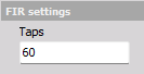
Taps
The number of Taps determines the steepness of the FIR LP-filtering. With an increased number of Taps the amplitude level will also have an increased low-pass attenuation rate at the cut-off frequency. For example, increasing the number of Taps to 600 from 60 will make the filter much more steep, as illustrated below:
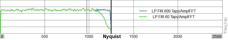
FIR filter cut-off frequency
The cut-off frequency used by the FIR decimation filters are set equal to the decimated Nyquist frequency, the sample rate divided by 2. For example if a channel with a 5 kHz sample rate is decimated with a factor of 2, then the LP-filtering will have a cut-off frequency at 2.5 kHz / 2 = 1.25 kHz, which is equal to the decimated Nyqust frequency.
At the cut-off frequency the LP-filtering will provide an attenuation of -3 dB.
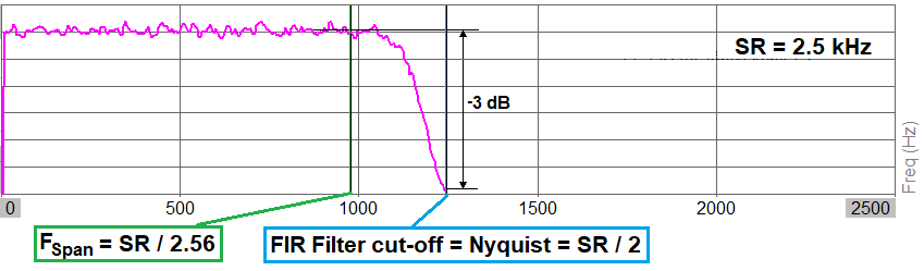
Note: The frequency at the sample rate divided by 2.56 is also referred to as the Frequency Span and is plotted on 2D graphs with a vertical line. This line can be seen if you zoom out the frequency axis to the Nyquist frequency.