Modal Circle
In structural dynamics, modal analysis is the process of determining a structure’s inherent dynamic characteristics—namely its natural frequencies, damping ratios, and mode shapes. To do this, engineers measure the structural response to a known excitation, generating a Frequency Response Function (FRF).
While an FRF is often viewed as a standard Bode plot (magnitude and phase versus frequency), plotting this same data in the complex plane unlocks a powerful and visually intuitive method for extracting modal parameters: the modal circle fit algorithm.
Here is a deep dive into how the modal circle works, the mathematics behind it, and how the algorithm extracts critical data from raw vibration signals.
The Theory Behind the Modal Circle
The foundation of the circle fit algorithm relies on analyzing a Single Degree of Freedom (SDOF) system. When a structure exhibits well-separated resonances, each mode of vibration can be treated mathematically as an independent SDOF system near its natural frequency.
If you plot the real part of $\alpha(\omega)$ on the X-axis and the imaginary part on the Y-axis—a representation known as a Nyquist plot—the locus of points as frequency sweeps through the resonance traces a near-perfect circle.
The Modal Circle widget is used for damping estimations of simple structures. Simple structures are here defined as structures with well separated modes (not overlapping modes) that can be treated as individual SDOF systems (Single Degree Of Freedom), similar to modes shown in the FRF graph example below:
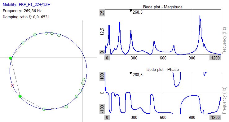
The Modal Circle widget determines the damping and resonance frequency based on an FRF channel (Frequency Response Function) and is therefore commonly used together with the Modal Test module, which calculates such FRF results.
FRF sample points laying around a resonance will be positioned in a circular pattern when seen on a Nyquist plot, which has a real and an imaginary axis. The Modal Circle widget shows such a Nyquist plot together with a circle fitted to those Fit points. The circular shape of points arises due to the phase changes that happen around resonances.
How the Circle Fit Algorithm Works
Data Selection and Circle Fitting
The algorithm first requires isolating a frequency band immediately surrounding a single resonance peak. Because measured FRF data contains noise and the influence of out-of-band modes, the selected points will not form a perfect mathematical circle.
The algorithm uses a least-squares mathematical regression to fit an ideal circle to the measured complex data points. This establishes the circle’s center coordinates and its radius, effectively filtering out random measurement noise.
Identifying the Natural Frequency ($\omega_r$)
On a modal circle, the frequency spacing between plotted points changes dramatically as you approach resonance.Far from resonance, points are clustered tightly together.As the frequency approaches the natural frequency, the arc length between consecutive frequency increments reaches its maximum.The algorithm identifies the natural frequency $\omega_r$ as the point on the fitted circle where the rate of change of phase angle with respect to frequency is maximized:$$\frac{d\theta}{d\omega} = \text{Maximum}$$Visually, this is the point where the data points are spread furthest apart.
Extracting the Damping Ratio ($\eta_r$)
Damping dictates how “wide” the resonance peak is, which translates geometrically to the angular distribution of points on the modal circle.To calculate the structural damping loss factor ($\eta_r$), the algorithm selects two data points, $\omega_a$ (below resonance) and $\omega_b$ (above resonance), and measures their angles $\theta_a$ and $\theta_b$ relative to the natural frequency point. The damping is calculated using the following exact relationship:$$\eta_r = \frac{\omega_b^2 - \omega_a^2}{\omega_r^2 (\tan\theta_a + \tan\theta_b)}$$For lightly damped systems, engineers frequently use the “half-power” points, where $\theta_a = \theta_b = 45^\circ$. In this specific case, the formula simplifies to the classic half-power bandwidth method:$$\eta_r \approx \frac{\omega_b - \omega_a}{\omega_r}$$
Determining the Modal Constant
The diameter of the fitted circle is directly proportional to the magnitude of the modal constant $_rA$, which is used to build the structure’s mode shapes. The orientation (phase angle) of the circle’s principal diameter indicates the phase of the mode shape, revealing whether a specific point on the structure is moving in-phase or out-of-phase with the excitation.
Widget Properties
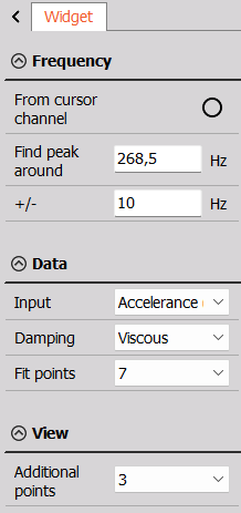
All widget parameter are described in the sections below:
From cursor channel
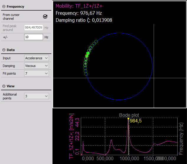
The yellow cursor on the 2D graph is taken for frequency point determination. When From cursor channel is enabled, you can use the yellow cursor in a 2D graph and set it around the frequency content of interest. The Modal Circle will find the nearest peak (resonance) and fit the circle into that data set. Then it will calculate the damping factor and more exact frequency (between line resolution of FFT).
Find peak around
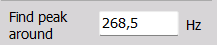
The Find peak around parameter is active when the From cursor channel is disabled. With Find peak around you can manually enter a frequency point for the circle fit procedure.
Peak search range (+/-)

The greatest peak in the defined frequency interval around the selected point will be used for the circle fit determination.
Input (physical quantity)
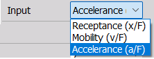
The Input type must be set in accordance with the physical quantity of the selected FRF channel. For example, if the used FRF channel has the unit [g / N] or [m/s^2 / N] then select Accelerance, which is the physical quantity for acceleration over force.
The selected Input must match the unit of the used channel in order to properly convert the channel into the domain where we need to fit the circle.
Damping and Resonance frequency calculations
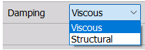
The DEWESoft Modal circle widget lets the user choose between a structural and a viscous damping model:
- The structural damping model is based on the receptance and calculates the damping loss factor, eta $[\eta]$.
- The viscous damping model is based on the mobility and calculates the damping ratio, zeta $[\zeta]$.
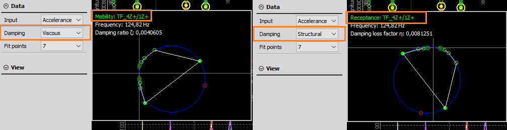
If the Input FRF channel has another physical quantity than the selected damping model uses, then the Modal Circle widget first automatically integrate or differentiate it to get the correct form.
Resonance frequency determination
To determine a resonance frequency $f_r$, first a circle is fitted to N number of FRF Fit points around an FRF resonance peak. Next, $f_r$ is determined by the fitted Circle center, the Complex plane origin position, and the two Fit points closest to the resonance frequency, one below $B$ and one above $A$ with respect to frequency:
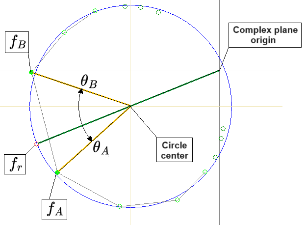
From the picture above, the determined Resonance frequency $f_r$ is marked with a red circle point. $f_r$ is found on the fitted blue circle at the position where the green line crosses over. The green line is a line going through the Complex plane origin and the fitted circle center.
Described with a formula this can be written as:
$$f_r= \frac{\theta_A \cdot f_B - \theta_B \cdot f_A}{\theta_A - \theta_B},$$
where points $A$ and $B$ are the points just After and just Before the resonance frequency. $f_A$ and $f_B$ are the frequencies of those points, and $\theta_A$ and $\theta_B$ are angles between the green line to $f_r$ and the orange lines from the Circle center to point $B$ and $A$.
Structural damping model
In a Structural damping model, the Receptance $\alpha(f)$ forms a perfect circle on the Nyquist plot. The receptance can be formulated as:
$$\alpha(f) = \frac{X(f)}{F(f)} = \frac{1}{4\pi^2f_r^2 \left(1- \left( \frac{f}{f_r} \right) ^2+i \eta_r \right)}$$
This receptance formula is used to determine the formula for the damping Loss factor $\eta_r$ of a mode, based on the Fit points $A$ and $B$ closest to $f_r$:
$$\text{Loss factor} = \eta_r = \frac{f_A^2 - f_B^2}{f_r^2 \cdot \left( \left| \text{tan} \left( \frac{\theta_A}{2} \right) \right| + \left| \text{tan} \left( \frac{\theta_B}{2} \right) \right| \right) }$$
Viscous damping model
For the Viscous damping model, we used the Nyquist plot of Mobility $Y(f)$ which in a similar manner then forms a circle-like curve around the resonance. The mobility can be formulated as:
$$Y(f) = \frac{\dot{X}(f)}{F(f)} = \frac{if}{2\pi f_r^2\left( 1 - \left( \frac{f}{f_r} \right)^2 + 2i \left( \frac{f}{f_r} \right) \zeta_r \right) }$$
This mobility formula is used to determine the formula for the Damping ratio $\zeta_r$ of a mode, based on the Fit points $A$ and $B$ closest to $f_r$:
$$ \zeta_r = \frac{f_A^2 - f_B^2}{2 f_r \left(f_A \cdot \left| \text{tan}\left(\frac{\theta_A}{2} \right) \right| + f_B \cdot \left| \text{tan} \left( \frac{\theta_B}{2} \right) \right| \right)}$$
Fit points
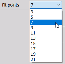
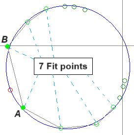
Select how many FRF sample points around the select frequency to use in total for the circle fit determination.
All used Fit points are marked with a light green circle edge, whereas the circle points $A$ and $B$ closest to $f_r$ are also filled out with that light green color:
Quadrants
When you plot a Frequency Response Function (FRF) on a complex plane (a Nyquist plot), the coordinate system is divided into four quadrants by the Real (X) and Imaginary (Y) axes.
The specific quadrant—or combination of quadrants—where the modal circle ends up is not random. It is dictated by a combination of the physical properties of the structure, your measurement setup, and the specific math of the FRF.
Here is a breakdown of what determines a modal circle’s position and orientation across the four quadrants.
The Baseline Rotation (FRF Type)
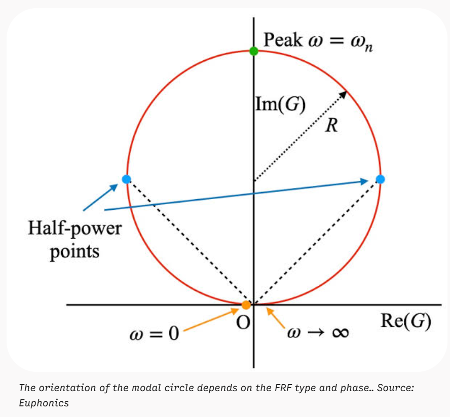
The parameter you choose to measure directly rotates the baseline circle in the complex plane by 90-degree increments. Assuming a perfect, isolated system measured at the driving point (where excitation and response are at the same location):
Receptance (Displacement / Force): The circle lies on the Negative Imaginary axis (spanning Quadrants III and IV).
Mobility (Velocity / Force): Differentiating displacement to velocity multiplies the function by $i\omega$. This rotates the circle 90° counter-clockwise, placing it on the Positive Real axis (spanning Quadrants I and IV).
- Accelerance (Acceleration / Force): Differentiating again rotates the circle another 90°, placing it on the Positive Imaginary axis (spanning Quadrants I and II).
Mode Shape Phase (The 180° Flip)
The phase of the mode shape determines whether a specific point on the structure moves in the same direction as your excitation force or in the opposite direction.
In-Phase (+): If the response point moves in the same direction as the force, the modal constant is positive, and the circle stays in its baseline position.
Out-of-Phase (-): If the response point moves in the opposite direction (e.g., the other side of a bending beam), the modal constant is negative. This multiplies the FRF by -1, flipping the circle 180 degrees into the exact opposite quadrant.
Complex Modes (The Tilt)
In textbook examples with “proportional damping” (where damping is distributed evenly across the structure), mode shapes are purely real numbers. The modal circle’s principal diameter will align perfectly with one of the axes.However, real structures often have non-proportional damping (e.g., a heavily damped joint on one side of a metal frame). This causes complex mode shapes, meaning different parts of the structure hit their maximum deflection at slightly different times.The visual result: The modal constant becomes a complex number, which tilts the circle away from the main axes. The circle might span diagonally across Quadrants I and III, for example. The angle of this tilt represents the phase angle of the complex mode shape.
Residuals (The Translation / Shift)
A true modal circle rarely starts exactly at the $(0,0)$ origin. The resonance you are analyzing is always slightly influenced by all the other modes in the structure.
Lower-frequency modes act as “residual mass” and push the circle along the axes.
Higher-frequency modes act as “residual stiffness” and pull the circle in the opposite direction.
The visual result: These out-of-band modes add constant Real and Imaginary offsets to your data. This physically shifts (translates) the entire circle left, right, up, or down. If the residual shift is large enough, an entire circle might be pushed entirely into a single off-axis quadrant (e.g., entirely inside Quadrant II)
Summary
When you look at a circle in specific quadrants, you are seeing a combination of Rotation (What are you measuring? Is it moving in or out of phase?), Tilt (Is the damping uneven, creating a complex mode?), and Translation (How hard are the other structural modes pushing or pulling on this specific resonance?).
Additional points
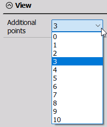
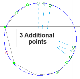
Select how many additional FRF points to show on the Nyquist plot. These points will not be used by the Modal circle widget for the determination of damping and resonance frequency, but can help indicate how uncoupled a mode is from other neighbor modes.
The Additional points are marked with a dark green circle edge, and the selected number of Additional points will be shown on each side of the resonance frequency.
References
- Modal Testing: Theory, Practice and Application, 2nd edition, year 2000, by D.J. Ewins, page 312-313.
- MODAL TESTING, Ostrava 2011, by Alena Bilošová, page 97, weblink:
https://moodle2.units.it/pluginfile.php/75129/mod_resource/content/1/EMA.pdf