Analog Sensors
DewesoftX offers an Analog sensor editor in which any already defined sensors and connected TEDS sensors will be listed automatically in a table.
You can find the following functions above the sensors table:
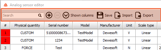
- Search
- Add/Remove
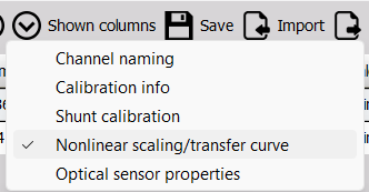
- Shown columns - Select which columns are visible
- Save - Saves the current configuration to AnalogSensors.dxb in the Dewesoft System folder
- Import - Import existing *.xml sensor databases
- Export - To a single file or each sensor separately
WARNING:It is not possible to restore deleted sensors.
Sensor Information
Each sensor is defined by the following information:
- General information
- Calibration
- Scaling type and parameters
- Optical sensor properties
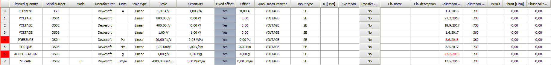
General Information
General information about the sensor will always be shown in the table:
- Physical quantity
- Serial number - Used for sensor identification, has to be unique.
- Model
- Manufacturer
- Unit - The electrical output unit of the sensor, most times V or A.
- Ampl. measurement - Amplifier measurement, the physical input unit that will be converted to an electrical unit.
- Input type
- R (Ohm)
- Excitation
- Min./Max. limit
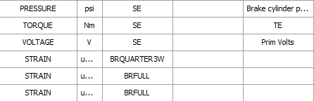
You can choose to show Channel naming:
- Channel name - Predefine the channel name for setup.
- Channel description - Additional information for easier identification.
Calibration
To see calibration information, enable Calibration info and/or Shunt calibration categories in Shown columns.
Sensor Calibration
You can configure the following information:
- Calibration date - Date of last calibration.
- Calibration period - How long the calibration is valid for, in days.
- Initials - Identify who performed the calibration.
Shunt Calibration
If using a shunt, you can modify:
- Shunt (Ohm) - Value of the shunt restance.
- Shunt cal target - target value for calibration, modify the allowed deviance from this target in Advanced Settings - Devices - Analog Input.
EXAMPLE:Using a shunt in Bridge operations for Strain gauges
Scaling
Dewesoft supports different scaling types within the sensor database. In addition to linear scaling, which can also be done in input channel setup, you can scale by the table or by the polynomial, as well as define transfer curves.
To change the scaling type from linear, enable Nonlinear scaling/transfer curve in Shown columns. Select the time domain scaling in the Scale type field, or enable the Transfer curve for frequency domain scaling.
Linear
Linear scaling is calculated by the formula:
$$y=kx + d$$
Where:
- $y$ = physical value
- $k$ = scale
- $x$ = measured value
- $d$= offset
Define the scale and offset in the sensors table:

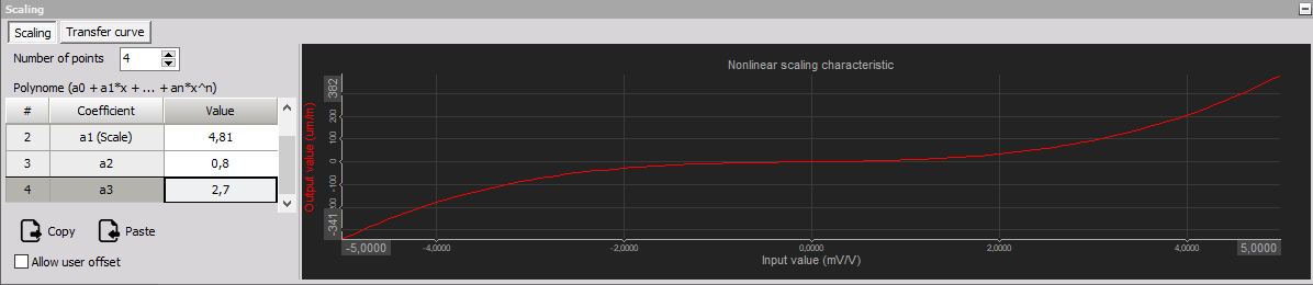
Polynome
Polynomial scaling is used for nonlinear sensors and it is calculated by the equation:
$$y = a_0 + a_1 x + a_2 x^2 + \ldots + a_n x ^n$$
Where: * $a_0$ - Offset * $a_1$ - Scale
You can Copy and Paste values to/from your clipboard. In order for the content to be pasted correctly, make sure to include the header Polynom first and the number of points last.
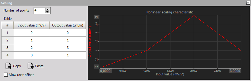
Table
Table scaling is also used for nonlinear sensors, but it is normally easier to enter because most calibration information contains several calibration points.
Enter the number of points (rows of the table) and in the table below, enter the X and Y values.
NOTE: If pasting values from a spreadsheet, the header row needs to be copied.
NOTE: As these three scaling types can’t compensate phase errors, they are used for time domain or angle based acquisitions. For frequency domain applications, a transfer curve will deliver more accurate results.
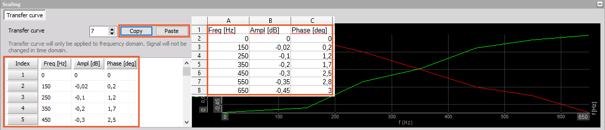
Transfer Curve
The transfer curve calibration can be used when the frequency behavior of the sensor is known:
- transfer curves for most common sensors are already measured,
- copy it from the calibration sheet of the sensor (if the calibration sheet includes the transfer curve),
- the third option is to measure it with Dewesoft FRF modal test, but this requires some additional equipment.
Some companies offer calibration reports for sensors also in the frequency domain, for example for current clamps. The transfer curve compensates amplitude and phase, both in relation to the signal frequency. In the table under Transfer curve column, we need to enter the points of the curve.
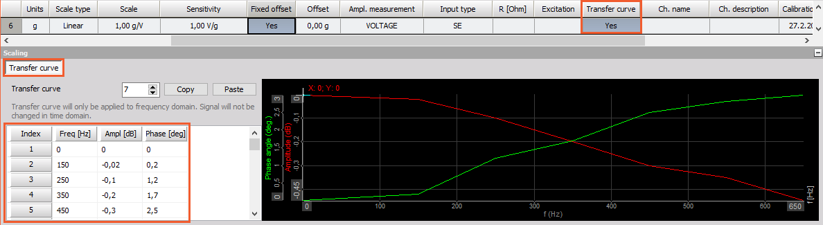
We can enter the sensors transfer curve in two ways:
- Manually enter the number of points (rows of the table) and in the numbers below the columns Freq [Hz] (signal frequency), Ampl [dB] (amplitude deviation) and Phase [deg] (phase angle).
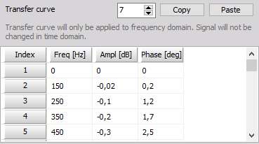
- Using the Windows copy and paste the values from a table created in the external program (e.g. Excel, …).
NOTE: Please keep in mind that the transfer curve is only helpful in frequency domain application (FFT, harmonics, octave analysis, …). You will not see the effect of sensors transfer curve in the time domain data - for that it is best to use a filter with similar characteristics like the transfer curve.