Classification

Classification is a procedure to count the values from the channel and puts them in the classes. A classical classification from the primary school is to create the classes and count number of student with specific weight or height.

Classification in measurement field is used for various applications, for example to find the distribution of power grid frequencies with time or to find the distribution of sound levels to which certain area or working place is exposed to.

First of all, we need to define what will be the result of classification. There are three options:

• Single value based - the result will be one array holding the result of the entire run
• Block based - the result will be set of the array each one added at the end of the defined block size. If we have for example 2 seconds block size and acquire data for 10 seconds, we will get 5 arrays of classification values, each valid for 2 seconds of data.
• Running - A running total is the summation of a sequence of numbers which is updated each time a new number is added to the sequence, by adding the value of the new number to the previous running total.
• Show class as a separate channel- option will create single value channels for each of the class element. This is a nice option to display the values in the multimeter.

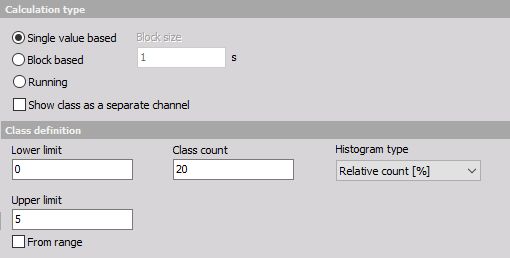
For class definition we need to set the:

• Lower limit - this will set the lower limit for start counting - all values below this level will be counted in the first class
• Upper limit - this will set the upper limit for an end of counting all values above this level will be counted in the last class
• Class count - defines the number of classes. In the example above the width of each class will be 5/20=0,25. First and last class will have half-width, so it will go from 0 to 0.125. The second class has a middle value of 0.25 and it goes from 0.125 to 0.375 and so on.

Histogram type defines what will be the output of the data (amplitude):

• Absolute count - each class value has the number of samples within the class (value will always count up)
• Relative count - each class value has the value of samples with the class normalized to the total number of counted samples (sum of all classes will be always 1)
• Relative count [%] - same as relative count, but expressed in percent (sum of all classes will be always 100)
• Density - provides empirical probability density each class value has the number of samples normalized to the total number of samples and divided by class width. In this case, the value is not depending on the number of classes within a range
• Density [%] - same as density but multiplied with 100
• Distribution - provides empirical probability distribution, each class value has the sum of all lower classes and the number of current samples, normalized to the total number of samples. The highest class has the value of 1.
• Distribution [%] - same as distribution, but expressed in percent. The highest class has the value of 100.

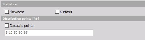
There are also several special output channels available. Two of them are Skewness (asymmetry of the probability distribution) and Kurtosis (a measure of “peakness” of distribution). Additionally, we can output a list of Distribution point values. Distribution points are the class values at which distribution reaches the entered value.

For the moment the distribution points work only if a distribution is chosen as the histogram type.

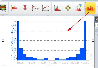
Histograms can be seen in the 2D graph during measurement and analysis.

If we choose block based calculation, we can also use the 3D graph to display the history of classifications.