Octave analysis
As opposed to FFT analysis, which has a specific number of lines per linear frequency (x axis), CPB (constant percentage bandwidth, called also octave) has a specific number of lines if logarithmic frequency x axis is used. Therefore lower frequencies have more lines than higher ones.
CPB analysis is traditionally used in sound and vibration field.
When you press the Setup button on CPB analysis math item, the following setup window will open:
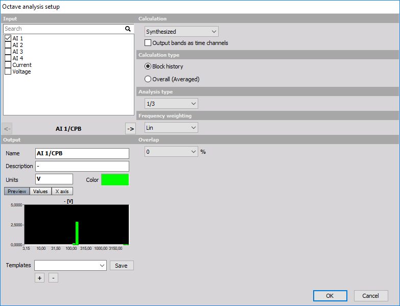
Calculation principle can be selected as a synthesized or true octave. Synthesized CPB is calculated using FFT as the base for calculating octave bands. Therefore it is updated only with every FFT being calculated.
True octave uses filters sets as in old analog (very expensive) octave analyzers. It uses more computing power and the result if only average spectrum over the entire run is needed is virtually the same. But when we observe that in real time, the difference is like night and day. We really see the dynamic behavior of the input data.
NOTE: True octave filters exactly represents the filter sets defined by the IEC 61260 standards and give the user real-time response for vivid live visualization of data, crucial for advanced acoustic analysis
Calculation type can be Overall (Averaged), where the result is one spectrum for the entire record.
The second option is Block history, where the CPBs are acquired shot by shot and put into the buffer. In this case, they can be observed on the 3D graph. The number of averages can be also set. When we enter a value of n, then it will calculate the average of n spectrum and put the result in the channel. Manual history count can override the normal settings for the number of shots to be kept in the memory during measurement.
Analysis type defines the number of bands within one octave. One octave means that the next center frequency of the band is twice the value of the current one. If we have 100 Hz, next octave band will be at 200 Hz. Then these octaves are further divided by a number defined in the analysis type field. 1/3 octave will have three bands per one octave and so on. So the higher the number is, more precise frequencies will be possible to observe and more calculation power will be used, especially with true octave.
Two additional fields must be defined if the true octave is used. First is Exponential averaging time, which defines the speed that the averaging filter works after each band is calculated. The three values correspond to the noise standard values (0.035 is IMPULSE, 0.125 sec is FAST, 1 sec is SLOW), other values can be also freely entered.
The second field is the Lower band frequency, which defines what will be the lowest value for calculation.
As all matrix channels also CPB can be best seen on the 2D graph. Block-based CPB can be also put in the 3D graph for viewing the history.
There is also an option, to define triggers in scope math when you would like to start the measurement and you don’t need to capture whole data for CPB.